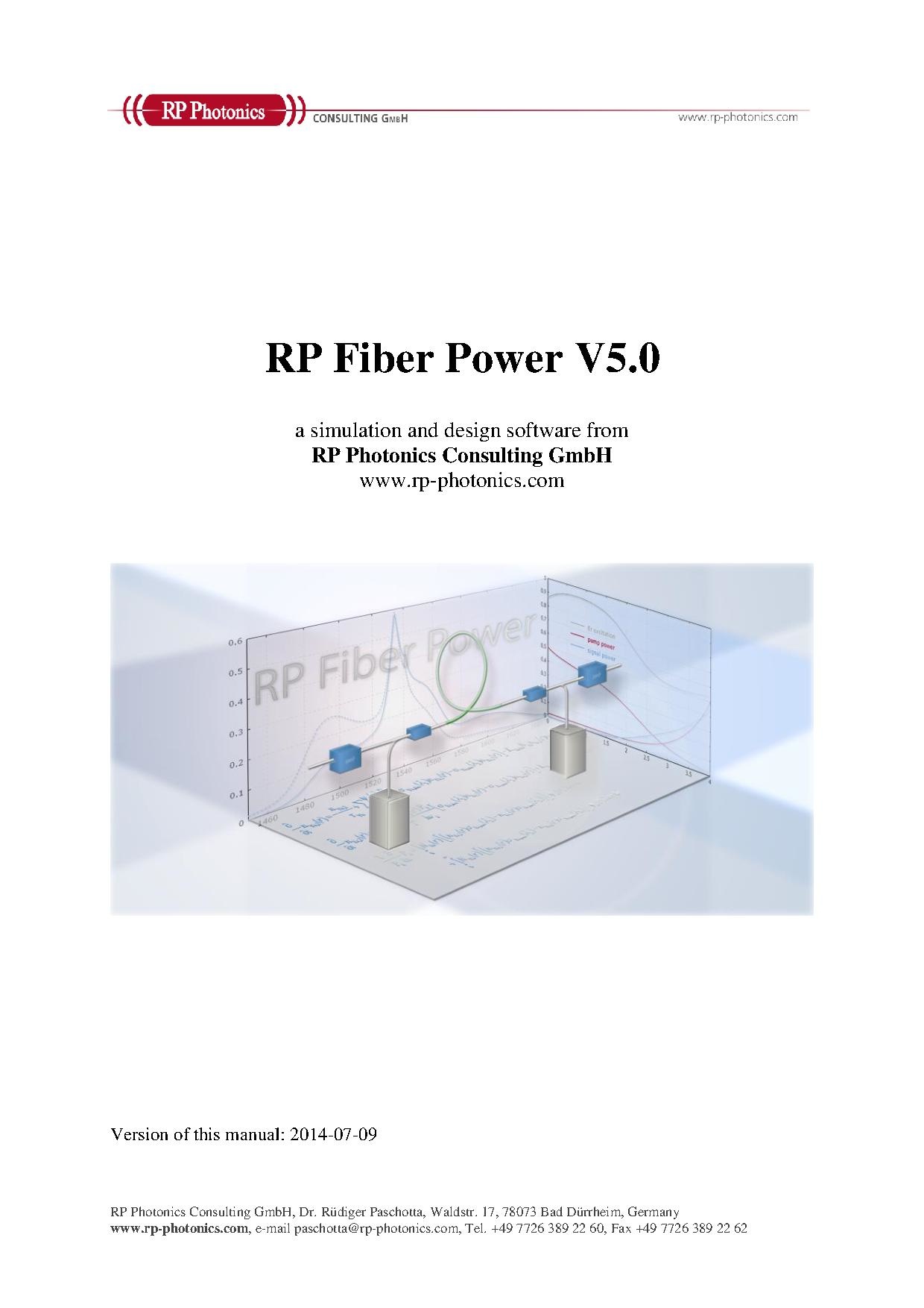
Fiber Simulations with RP Fiber Power
RP Fiber Power 6
RP Fiber Power is a script based simulation software with a minimal GUI for basic functions designed by Dr. Rüdiger Paschotta.
Website:
Comprehensive User Manual:
Simulating using GUI
After opening the software there are multiple tabs displayed in form mode. Each of these tabs provide information for various graphical outputs, but the ones we were particularly interested in were the simulations related to power efficiency in the active length of fiber.
Here we began inputting data into the Active tab. The amount of active fiber in use was put in the length section. Number of steps in the z-direction corresponds to the resolution of the output, the more steps, the higher the resolution and longer the computation time. According the RP Fiber Power user manual, one way to determine a value for the resolution is sufficient is to run the script once with an order of magnitude higher and see if there is a difference. If there is no visible difference, then the number of steps is sufficient. If the parameters for the fiber are correctly set and defined in a text file, the parameters of your specific fiber may be left in terms of variables to later be filled in by the software. You are able to choose from a variety of fibers in the drop down at the bottom of the tab, or load a custom text file by placing it in the same directory as the other fiber data. If uploading a custom file, make sure to define all variables or be diligent about including all values in the GUI.

Next, we look at the Optical Channels tab. This is where information about your pump and signal wavelength and power can be edited along with the amplified spontaneous emission (ASE). In the GUI, you are able to input information about two pumps and two signals, though if a more complex set up is in use, more inputs and outputs can be added. If working with a simple system, only a few paramters in each tab need to be edited. This includes the operating wavelength and the input power. In this screencap, there is a small error, the intensity profile should be set as Gaussian.

This tab is very similar to the previous pump tab. It may be useful to note that no input power is necessary unless you have external energy coming into your system at the signal point.

Here you are able to see the wavelength range at which your active fiber can emit amplified spontaneous emission. The wavelength range define here is the range of the corresponding output graph. The step length corresponds to the resolution of the output. The number of propagation modes can be varied to simulate a real or ideal system.

Again we switch tabs, this time to the Graphics tab. Here you are able to select a variety of graphs that the software will output upon running the script. For this example we selected three graphs to display, power versus position, an ideal case of fiber length versus pump and signal power, and the ASE spectrum.
You are able to select which signal to display here. Though in this case we chose to view only the pump and signal power for the specified length of active fiber.

Here we are able to view the behavior of the pump and signal strength past what is observed on the Pump vs. Power graph. This graph can model any length of active fiber, to get an idea of how a particular system might behave over a long distance.


Understanding the ASE, both in the middle of the fiber and at the end of the fiber, helps to understand extra noise in spectrum measurements.

This is an ideal setup. Though there would be other issues with having this length of active fiber, it is still good to understand the relationship between the pump and signal power over a long span.

Here is the corresponding script for the input that is outlined above. It may be helpful to go over line by line to gain an understanding of what calculations are made to display these graphs.

Simulating with a Script
hello