Difference between revisions of "Machine Learning: Linear Regression"
Aplstudent (talk | contribs) |
Aplstudent (talk | contribs) |
||
| Line 6: | Line 6: | ||
<code> | <code> | ||
import numpy as np | import numpy as np | ||
| + | |||
| + | |||
import matplotlib.pyplot as plt | import matplotlib.pyplot as plt | ||
| + | |||
| + | |||
pair=np.array([(1,1),(4,4.2),(2,2)]) | pair=np.array([(1,1),(4,4.2),(2,2)]) | ||
| + | |||
| + | |||
</code> | </code> | ||
| Line 19: | Line 25: | ||
nepoch = 4 | nepoch = 4 | ||
| + | |||
| + | |||
m=0.0 | m=0.0 | ||
| + | |||
| + | |||
b=0.0 | b=0.0 | ||
| + | |||
| + | |||
alpha = 0.2 | alpha = 0.2 | ||
| + | |||
| + | |||
</code> | </code> | ||
| − | each pair is looped through and a y is predicted according to <math> | + | each pair is looped through and a y is predicted according to <math>Ypred=X*m+b</math> The error is then found according to <math>Ypred-Y</math> The weights are then updated according to the formula <math>m:=m-learning_rate*error*x</math> and <math>b:=b-learning_rate*error</math> The new value of the paramaters are used with the next set of points. |
<code> | <code> | ||
Revision as of 01:05, 12 November 2016
Machine learning is the subfield of Artificial intelligence interested in making agents that review their past actions and experiences to formulate a new action. The task is to learn the formula for a function. A performance standard is used to adjust the function that is predicted. Linear regression is a common pattern that can be approximated by learning the parameters for slope and intercept.
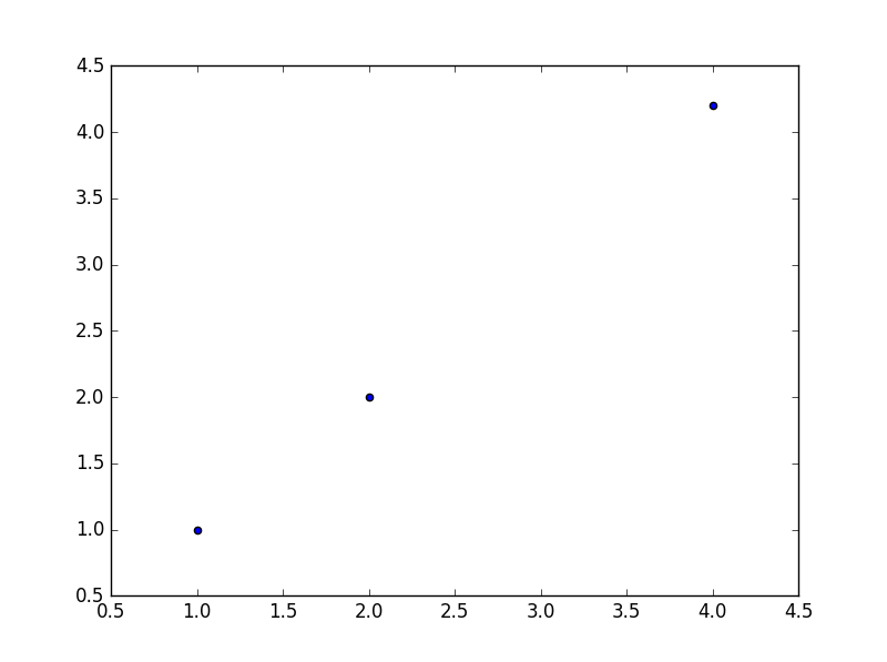
Here are the packages that are used and three points to approximate a function from.
import numpy as np
import matplotlib.pyplot as plt
pair=np.array([(1,1),(4,4.2),(2,2)])
The slope and intercept must be initialized by the user. In addition the learning rate is how quickly to change the parameters by each iteration. the data set is fitted multiple times with updated starting weights, these are epochs.
nepoch = 4
m=0.0
b=0.0
alpha = 0.2
each pair is looped through and a y is predicted according to The error is then found according to The weights are then updated according to the formula and The new value of the paramaters are used with the next set of points.
for i in range(0,nepoch,1):
   print("i=" , i)
   for i in [0,1,2]:
       print(m,b)
       x=pair[i][0]
       y=pair[i][1]
       y_pred=m*x+b
       error=y_pred-y
       m=m-alpha*error*x
       b=b-alpha*error
   print(m,b)
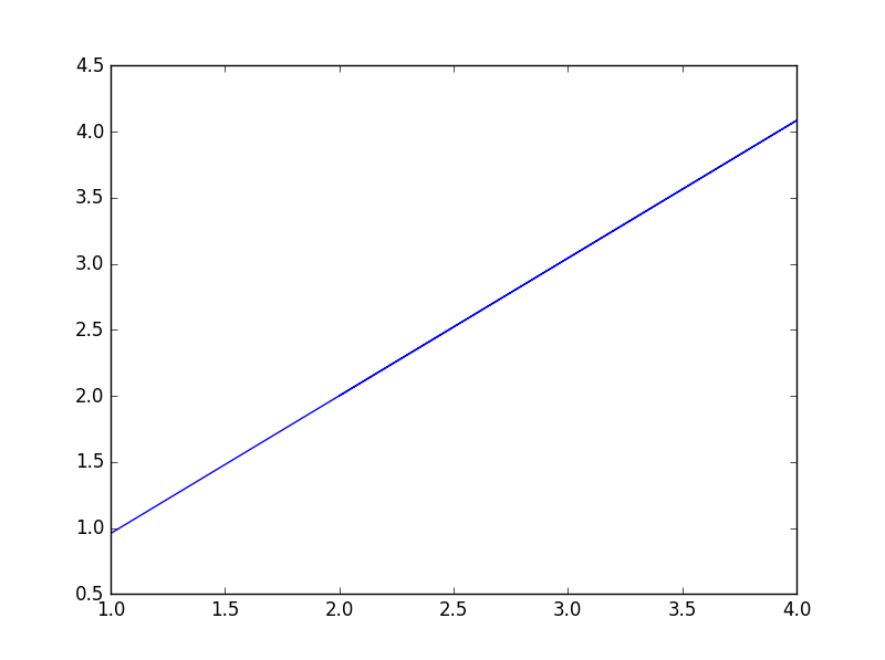
the slope is found to be 1.04 and the y-intercept as -0.08. Imperfect data was used so the exact value was not found. The choice of alpha is important because a value that is too large will give an erroneous result. The algorithm will overshoot the exact value and then update it by overshooting it again resulting in the answer revolving around the exact value.


