Difference between revisions of "Fiber Simulations with RP Fiber Power"
(→Simulating using GUI) |
|||
| (36 intermediate revisions by one other user not shown) | |||
| Line 1: | Line 1: | ||
| − | + | = RP Fiber Power 6 = | |
| − | RP Fiber Power is a script based simulation software | + | RP Fiber Power is a script based simulation software designed by Dr. Rüdiger Paschotta. The software has a fairly minimal GUI but custom scripts can be written to simulate nearly any fiber system. For examples of possible simulations outside of the basic options, look at the demo folder (placed in the documents section of the computer with RP Fiber Power installed). A more detailed description of any of the demonstration scripts can be found the in the RP Fiber Power user manual. |
[https://www.rp-photonics.com/fiberpower.html RP Fiber Power Website] | [https://www.rp-photonics.com/fiberpower.html RP Fiber Power Website] | ||
| − | + | ||
| + | = Simulating Using the Provided GUI = | ||
| + | |||
| + | == Input Tabs == | ||
After opening the software there are multiple tabs displayed in form mode. Each of these tabs provide information for various graphical outputs, but the ones we were particularly interested in were the simulations related to power efficiency in the active length of fiber. | After opening the software there are multiple tabs displayed in form mode. Each of these tabs provide information for various graphical outputs, but the ones we were particularly interested in were the simulations related to power efficiency in the active length of fiber. | ||
| − | Here we began inputting data into the Active tab. The amount of active fiber in use was put in the length section. | + | Here we began inputting data into the 'Active' tab. The amount of active fiber in use was put in the length section. |
Number of steps in the z-direction corresponds to the resolution of the output, the more steps, the higher the resolution and longer the computation time. According the RP Fiber Power user manual, one way to determine a value for the resolution is sufficient is to run the script once with an order of magnitude higher and see if there is a difference. If there is no visible difference, then the number of steps is sufficient. If the parameters for the fiber are correctly set and defined in a text file, the parameters of your specific fiber may be left in terms of variables to later be filled in by the software. You are able to choose from a variety of fibers in the drop down at the bottom of the tab, or load a custom text file by placing it in the same directory as the other fiber data. If uploading a custom file, make sure to define all variables or be diligent about including all values in the GUI. | Number of steps in the z-direction corresponds to the resolution of the output, the more steps, the higher the resolution and longer the computation time. According the RP Fiber Power user manual, one way to determine a value for the resolution is sufficient is to run the script once with an order of magnitude higher and see if there is a difference. If there is no visible difference, then the number of steps is sufficient. If the parameters for the fiber are correctly set and defined in a text file, the parameters of your specific fiber may be left in terms of variables to later be filled in by the software. You are able to choose from a variety of fibers in the drop down at the bottom of the tab, or load a custom text file by placing it in the same directory as the other fiber data. If uploading a custom file, make sure to define all variables or be diligent about including all values in the GUI. | ||
[[File:Active.png|500px]] | [[File:Active.png|500px]] | ||
| + | |||
| + | Next, we look at the 'Optical Channels' tab. This is where information about your pump and signal wavelength and power can be edited along with the amplified spontaneous emission (ASE). In the GUI, you are able to input information about two pumps and two signals, though if a more complex set up is in use, more inputs and outputs can be added. If working with a simple system, only a few paramters in each tab need to be edited. This includes the operating wavelength and the input power. In this image, there is a small error, the intensity profile should be set as Gaussian. | ||
[[File:Pump.png|500px]] | [[File:Pump.png|500px]] | ||
| + | |||
| + | This tab is very similar to the previous pump tab. It may be useful to note that no input power is necessary unless you have external energy coming into your system at the signal point. | ||
[[File:Signal.png|500px]] | [[File:Signal.png|500px]] | ||
| + | |||
| + | Here you are able to see the wavelength range at which your active fiber can emit amplified spontaneous emission. The wavelength range define here is the range of the corresponding output graph. The step length corresponds to the resolution of the output. The number of propagation modes can be varied to simulate a real or ideal system. | ||
[[File:Ase.png|500px]] | [[File:Ase.png|500px]] | ||
| + | |||
| + | Again we switch tabs, this time to the 'Graphics' tab. Here you are able to select a variety of graphs that the software will output upon running the script. For this example we selected three graphs to display, power versus position, an ideal case of fiber length versus pump and signal power, and the ASE spectrum. | ||
| + | |||
| + | You are able to select which signal to display here. Though in this case we chose to view only the pump and signal power for the specified length of active fiber. | ||
[[File:Powervsposition.png|500px]] | [[File:Powervsposition.png|500px]] | ||
| + | |||
| + | Here we are able to view the behavior of the pump and signal strength past what is observed on the 'Pump vs. Power' graph. This graph can model any length of active fiber, to get an idea of how a particular system might behave over a long distance. | ||
[[File:Variationoffiberlength.png|500px]] | [[File:Variationoffiberlength.png|500px]] | ||
| + | |||
| + | |||
| + | == Output Graphs == | ||
| + | |||
| + | Here is the standard pump versus signal graph corresponding to designated active fiber length from the 'Active' tab. | ||
[[File:Final_active_fiber_length.png|500px]] | [[File:Final_active_fiber_length.png|500px]] | ||
| + | |||
| + | This is an ideal setup. Though there would be other issues with having this length of active fiber, it is still good to understand the relationship between the pump and signal power over a long span. | ||
| + | |||
| + | [[File:Variation_of_fiber_length.png|500px]] | ||
| + | |||
| + | Understanding the ASE, both in the middle of the fiber and at the end of the fiber, helps to understand extra noise in spectrum measurements. | ||
[[File:Functional_ase.png|500px]] | [[File:Functional_ase.png|500px]] | ||
| − | |||
| − | == Simulating with a Script == | + | == Background Script == |
| + | |||
| + | |||
| + | Here is the corresponding script for the input that is outlined above. It may be helpful to go over line by line to gain an understanding of what calculations are made to display these graphs. This can be viewed by selecting the 'Show Editors' button. | ||
| + | |||
| + | [[File:Pumpscript.png|1500px]] | ||
| + | |||
| + | = Simulating with a Script = | ||
| + | |||
| + | After becoming familiar with the interface to build some basic optical systems such as the power amplifier above, a deeper look into the managed code of RP Fiber Power will demonstrate the variety of applications for which it can be applied. In this example, we model the pump absorption in a double-clad fiber to show the necessary of mode-scrambling in the power amplifier. | ||
| + | |||
| + | Begin by defining the wavelength of the pump and the properties of a double-clad fiber. In this case, we use an erbium-ytterbium doped fiber from [http://www.nufern.com/pam/optical_fibers/979/SM-EYDF-6_125-HE/ Nufern]. Here, the core radius is 3 micrometers, the cladding radius is 62.5 micrometers and the numerical apertures of the core and cladding are 0.18 and 0.46 respectively. We also define the index and the V number of the core and cladding. If working with different fiber designs, such as a D-shaped inner cladding, one can implement them into the refractive index profile by defining a limitation. In our case, we leave the cut, but set it equal to the radius of the inner cladding. | ||
| + | |||
| + | [[File:DefiningtheFiber.png|500px]] | ||
| + | |||
| + | The refractive index profile is constructed defining a variable for the radius and using an "if-then" statement which sets the index equal to the index of the core for when the radius is less than or equal to r_cor. Consequently, if the radius is greater than r_cor and less than the cut we defined above as y_cut, then the index is equal to the index of the cladding. | ||
| + | Similarly, the loss in the fiber is constructed by defining the loss in the core and a function for the loss in the cladding in terms of the radius. Using another "if-then" statement, the loss is set equal to the loss in the core for when the radius is less than or equal to r_cor, and the loss in the outer cladding is equal to (in our case) 1e3*(r-r_cl)/(10 um) for when the radius is grater than the inner cladding (r_cl). | ||
| + | |||
| + | Before setting the grid parameters for the beam propagation, values can be set to be displayed in the output window by the "show" command. For example, we wish to display the core radius, cladding radius, numerical apertures, and V numbers below: | ||
| + | |||
| + | [[File:outputwindow.png|150px]] | ||
| + | |||
| + | It is now time to set the grid parameters that will determine the resolution, number of steps, and length of the fiber for the beam propagation. Define the maximum radius to be larger than the cladding to ensure the entire width of the cladding is taken into account. The number of points in the x and y direction of the fiber is taken to be large to ensure sufficient calculation and is set at 2^7. The spatial resolution is defined as the maximum radius divided by the number points in the x and y direction. We take the maximum z to be the total length of the fiber, remembering that the default unit in RP Fiber Power is meters. In our case, we set z_max:= 3000 mm with a longitudinal resolution of dz:=10 mm. The number of steps in the z direction is taken to be the total fiber length divided by the longitudinal resolution. Finally, the number of sub-steps at each dz can be set for further resolution in the z direction. Recognize that the more sub-steps involved for each dz will drastically increase the calculation time of the software. | ||
| + | |||
| + | To model the incident beam profile, we begin by defining the beam size parameter and the normalized super-Gaussian function. The calculation for the beam profile requires a for loop that is quite involved, but a case study on the simulation with the loop can be found on the [https://www.rp-photonics.com/fiberpower_dcf.html RP Photonics software website]. | ||
| + | |||
| + | The last step is to calculate the beam propagation which combines everything that has been written to this point. We begin the calculation by setting the grid parameters, the index profile, the loss profile, initial amplitude, interpolation and increased anti-aliasing of the index profile. | ||
| + | [[File:propagation.png|400px]] | ||
| + | |||
| + | We can graph the results of the field amplitude in the yz plane by setting diagram 1 with x axis from 0 to the fiber length x: 0, zmax/mm and the y axis from the bottom of the cladding to the top of the cladding y:-r_max/um to +r_max/um. The colors of both the loss and the power are set and information about the transmission can be portrayed on the graph by inserting the incident power transmission function in brackets, for example. The follow code and the graph output are displayed below. | ||
| − | + | [[File:graphcode.png|500px]] | |
| + | [[File:absorption.png|500px]] | ||
Latest revision as of 10:02, 17 August 2022
Contents
RP Fiber Power 6
RP Fiber Power is a script based simulation software designed by Dr. Rüdiger Paschotta. The software has a fairly minimal GUI but custom scripts can be written to simulate nearly any fiber system. For examples of possible simulations outside of the basic options, look at the demo folder (placed in the documents section of the computer with RP Fiber Power installed). A more detailed description of any of the demonstration scripts can be found the in the RP Fiber Power user manual.
Simulating Using the Provided GUI
Input Tabs
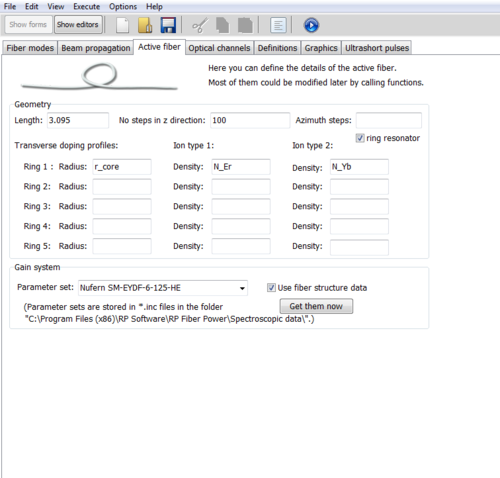
After opening the software there are multiple tabs displayed in form mode. Each of these tabs provide information for various graphical outputs, but the ones we were particularly interested in were the simulations related to power efficiency in the active length of fiber.
Here we began inputting data into the 'Active' tab. The amount of active fiber in use was put in the length section. Number of steps in the z-direction corresponds to the resolution of the output, the more steps, the higher the resolution and longer the computation time. According the RP Fiber Power user manual, one way to determine a value for the resolution is sufficient is to run the script once with an order of magnitude higher and see if there is a difference. If there is no visible difference, then the number of steps is sufficient. If the parameters for the fiber are correctly set and defined in a text file, the parameters of your specific fiber may be left in terms of variables to later be filled in by the software. You are able to choose from a variety of fibers in the drop down at the bottom of the tab, or load a custom text file by placing it in the same directory as the other fiber data. If uploading a custom file, make sure to define all variables or be diligent about including all values in the GUI.
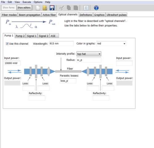
Next, we look at the 'Optical Channels' tab. This is where information about your pump and signal wavelength and power can be edited along with the amplified spontaneous emission (ASE). In the GUI, you are able to input information about two pumps and two signals, though if a more complex set up is in use, more inputs and outputs can be added. If working with a simple system, only a few paramters in each tab need to be edited. This includes the operating wavelength and the input power. In this image, there is a small error, the intensity profile should be set as Gaussian.
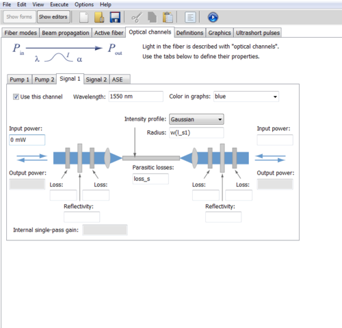
This tab is very similar to the previous pump tab. It may be useful to note that no input power is necessary unless you have external energy coming into your system at the signal point.
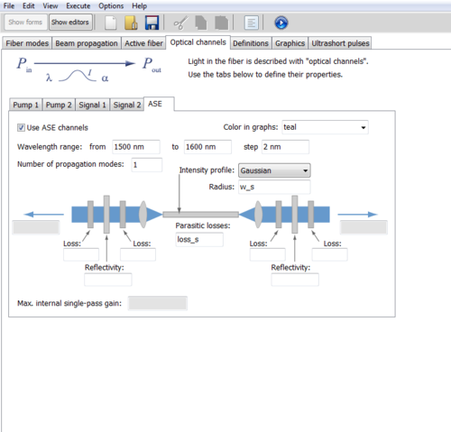
Here you are able to see the wavelength range at which your active fiber can emit amplified spontaneous emission. The wavelength range define here is the range of the corresponding output graph. The step length corresponds to the resolution of the output. The number of propagation modes can be varied to simulate a real or ideal system.
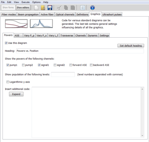
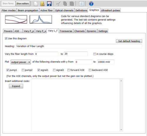
Again we switch tabs, this time to the 'Graphics' tab. Here you are able to select a variety of graphs that the software will output upon running the script. For this example we selected three graphs to display, power versus position, an ideal case of fiber length versus pump and signal power, and the ASE spectrum.
You are able to select which signal to display here. Though in this case we chose to view only the pump and signal power for the specified length of active fiber.
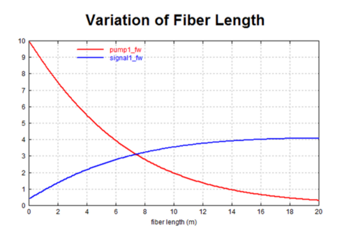
Here we are able to view the behavior of the pump and signal strength past what is observed on the 'Pump vs. Power' graph. This graph can model any length of active fiber, to get an idea of how a particular system might behave over a long distance.
Output Graphs
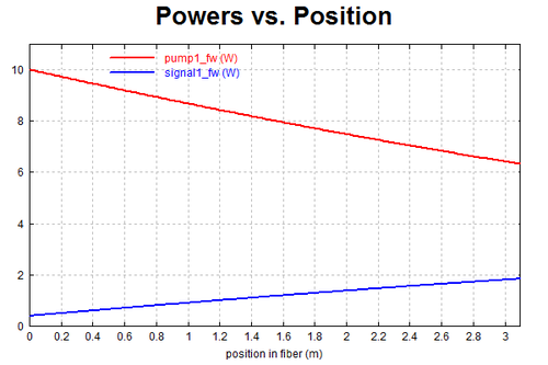
Here is the standard pump versus signal graph corresponding to designated active fiber length from the 'Active' tab.
This is an ideal setup. Though there would be other issues with having this length of active fiber, it is still good to understand the relationship between the pump and signal power over a long span.
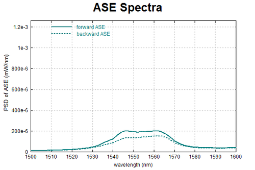
Understanding the ASE, both in the middle of the fiber and at the end of the fiber, helps to understand extra noise in spectrum measurements.
Background Script
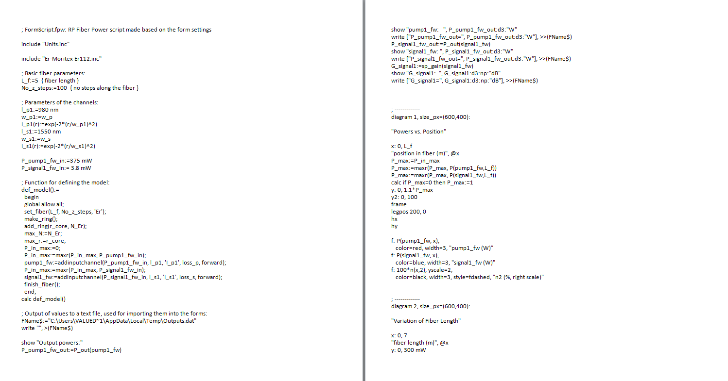
Here is the corresponding script for the input that is outlined above. It may be helpful to go over line by line to gain an understanding of what calculations are made to display these graphs. This can be viewed by selecting the 'Show Editors' button.
Simulating with a Script
After becoming familiar with the interface to build some basic optical systems such as the power amplifier above, a deeper look into the managed code of RP Fiber Power will demonstrate the variety of applications for which it can be applied. In this example, we model the pump absorption in a double-clad fiber to show the necessary of mode-scrambling in the power amplifier.
Begin by defining the wavelength of the pump and the properties of a double-clad fiber. In this case, we use an erbium-ytterbium doped fiber from Nufern. Here, the core radius is 3 micrometers, the cladding radius is 62.5 micrometers and the numerical apertures of the core and cladding are 0.18 and 0.46 respectively. We also define the index and the V number of the core and cladding. If working with different fiber designs, such as a D-shaped inner cladding, one can implement them into the refractive index profile by defining a limitation. In our case, we leave the cut, but set it equal to the radius of the inner cladding.
The refractive index profile is constructed defining a variable for the radius and using an "if-then" statement which sets the index equal to the index of the core for when the radius is less than or equal to r_cor. Consequently, if the radius is greater than r_cor and less than the cut we defined above as y_cut, then the index is equal to the index of the cladding. Similarly, the loss in the fiber is constructed by defining the loss in the core and a function for the loss in the cladding in terms of the radius. Using another "if-then" statement, the loss is set equal to the loss in the core for when the radius is less than or equal to r_cor, and the loss in the outer cladding is equal to (in our case) 1e3*(r-r_cl)/(10 um) for when the radius is grater than the inner cladding (r_cl).
Before setting the grid parameters for the beam propagation, values can be set to be displayed in the output window by the "show" command. For example, we wish to display the core radius, cladding radius, numerical apertures, and V numbers below:
It is now time to set the grid parameters that will determine the resolution, number of steps, and length of the fiber for the beam propagation. Define the maximum radius to be larger than the cladding to ensure the entire width of the cladding is taken into account. The number of points in the x and y direction of the fiber is taken to be large to ensure sufficient calculation and is set at 2^7. The spatial resolution is defined as the maximum radius divided by the number points in the x and y direction. We take the maximum z to be the total length of the fiber, remembering that the default unit in RP Fiber Power is meters. In our case, we set z_max:= 3000 mm with a longitudinal resolution of dz:=10 mm. The number of steps in the z direction is taken to be the total fiber length divided by the longitudinal resolution. Finally, the number of sub-steps at each dz can be set for further resolution in the z direction. Recognize that the more sub-steps involved for each dz will drastically increase the calculation time of the software.
To model the incident beam profile, we begin by defining the beam size parameter and the normalized super-Gaussian function. The calculation for the beam profile requires a for loop that is quite involved, but a case study on the simulation with the loop can be found on the RP Photonics software website.
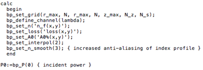
The last step is to calculate the beam propagation which combines everything that has been written to this point. We begin the calculation by setting the grid parameters, the index profile, the loss profile, initial amplitude, interpolation and increased anti-aliasing of the index profile.
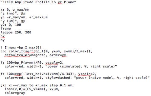
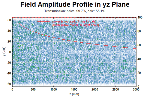
We can graph the results of the field amplitude in the yz plane by setting diagram 1 with x axis from 0 to the fiber length x: 0, zmax/mm and the y axis from the bottom of the cladding to the top of the cladding y:-r_max/um to +r_max/um. The colors of both the loss and the power are set and information about the transmission can be portrayed on the graph by inserting the incident power transmission function in brackets, for example. The follow code and the graph output are displayed below.
